 and
and 
where:
 = total distance of the low-cost carrier in kilometres
 = total number of low-cost carrier flights
 = total travel time of the low-cost carrier in minutes
In a previous section seven characteristics of flight routes have been discussed: distance, density, frequency, connectivity, concentration, geographic direction, competition, network development, and hierarchy. In this part these characteristics will be operationalized with the aim to describe the network morphology and development (click on a link to jump to the related subject). The different characteristics of flight routes will mostly be analysed for each low-cost carrier type, and aggregated at the low-cost carrier types.
The distance of flight routes is the distance between origin and destination of a flight and will be given in kilometers and minutes. It can be calculated how much a low-cost carrier travelled on average by flight and by route. The average distance in kilometres and respectively minutes can be calculated as follows:
and
where:
= total distance of the low-cost carrier in kilometres
= total number of low-cost carrier flights
= total travel time of the low-cost carrier in minutes
By dividing the total distance in kilometres with the total number of flights the average distance can be calculated. The average travel time is calculated by dividing the total travel time with the total number of flights.

The Eta index calculates the average distance for each route by dividing the total length of the routes with the total number of routes. Click here for more information about this index.
By analyzing the density of different routes more understanding can be obtained about the location of the more busier routes. In this research the density of routes is determined by looking at the absolute number of seats on a route between origin and destination. Next to the number of seats this can also be done with the number of flights. The density for a flight route from location A to destination B is defined as:

where:
 = total number of seats at route AB
These densities will be visualised using GIS over the period 1990 – 2005. This way the network development of a low-cost carrier can be analysed.
With frequency the flight frequency is meant. Both the total and average number of low-cost carrier flights will be analysed. Flight frequency data can be obtained almost directly from the OAG database.
In this research connectivity will be defined as the average number of connections at an airport in a low-cost carrier network. This can be operationalized by looking at the number of flight routes at an airport for each of the selected low-cost carriers. This way an overview can be created of the connectedness of airports within the selected low-cost carrier network. The degree of connectivity can be obtained through the beta index:

The beta index is calculated by dividing the total number of routes with the total number of airports. The graph section gives a description of this index. Because the flights are return flights, the lowest possible beta value is 1.
To get a better understanding of the spatial concentration within a network a concentration measure can be used. There are different concentration measures available to analyse the spatial concentration. Examples of these measures are the McShan-Windle index, Herfindahl index, Entropy index, Theil index, variation coefficient, and the Gini index. From research of Burghouwt (2003), Reynolds-Feighan (2001), and Wojahn (2001) it appears the Gini index is the most correct measure to analyse the concentration of different carrier networks. The Gini index can be defined as:
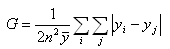
where:
y = the air traffic at airport i or j, measured in available seats
n = the number of airports within a network
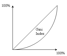
The result of the Gini index will look like a Lorenz curve (figure 20). The diagonal is the result when all traffic has been divided equally over the network and the Gini index has a value of 0. The larger the Gini index, the more the result will look like a Lorenz curve, and the more the traffic will be divided unequally over the network.
| Figure 20, Lorenz curve Gini index |
 |
The time dimension is important when analyzing the network development. The network development will be analysed for each carrier during the period 1990 – 2005. At different points in time maps will be created at which the network of a selected carrier will be visualized. Routes will be visualized proportionally depending on the seat density of the related route. By showing the different maps one after the other a slideshow can be created displaying the network development. The network development of each carrier can be found here.
When visualizing the network with help of a GIS the geographical direction will also be analyzed. It is possible a certain direction can be strongly represented for a certain low-cost carrier type. For example a network could have a North-South or East-West direction. To analyse the direction five regions will be defined, allowing 25 possible flight directions. At each direction will be looked at the percentage of seats.
In this research competition can be measured by looking at doubling routes. One speaks of a doubling route if two or more carriers operate on the same route, for example when two different carriers operate between Amsterdam Schiphol and London Heathrow. The four low-cost carrier types could double with other low-cost carriers or with full-service carriers. Because full-service carriers operate according to a hub-and-spoke system (in contrary to a low-cost carrier which operate according to a point-to-point system), they could double directly, and indirectly with a stop over. Doubling routes can be found with help of GIS programs.
To get an indication of the amount of competition on low-cost carriers the number of available seats will be used. Competition can be defined as:

where:
 = total number of competing seats
 = total number of seats
Competition can be analyzed for all low-cost carriers. Competition will be visualized with GIS programs.